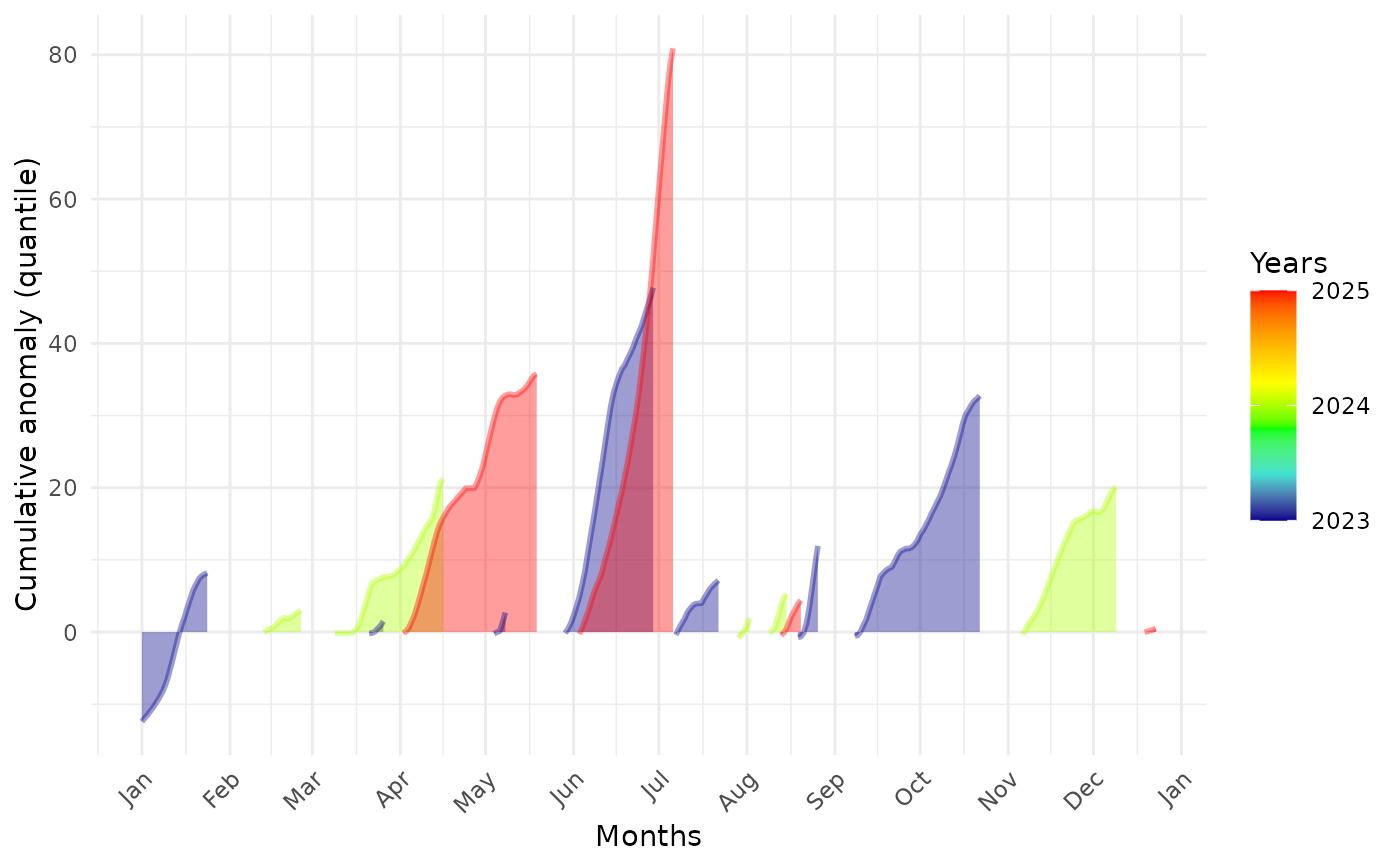
Cumulative anomaly against months of the years

Allows to see at which time of the year a place is explosed to the bigest anomalies.

BEE.plot.cumulative_anomaly(
  metric_point_df,
  start_date = NULL,
  end_date = NULL,
  ...
)

Arguments

metric_point_df

: The output of BEE.calc.metric_point() for a given location. Please note that the output of BEE.calc.metric_point() is a list. You only need to provide a dataframe from that list, not the whole list.

start_date

: = NULL by default or the date at which you want to start the plot. It must be in the same format than metric_point_df$date.

end_date

: = NULL by default or the date at which you want to stop the plot. It must be in the same format than metric_point_df$date.

...

: Customising the graph is possible by adding any general ggplot2 argument.

Value

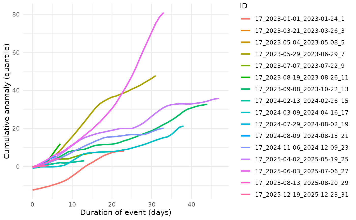
A 'ggplot2' with the months on the x-axis, the cumulative anomaly per extreme event of the studied parameter value on the y-axis.

Examples

# Load data:
file_name_1 <- system.file(file.path("extdata", "metrics_points_pixel.rds"),
                                  package = "BioExtremeEvent")
metrics_points_day <- readRDS(file_name_1)
# Get data set for one gps point
metrics_points_day <- metrics_points_day[[1]] # first gps point
BEE.plot.cumulative_anomaly(metric_point_df = metrics_points_day,
                    start_date = NULL,
                    end_date = NULL)