4. Calculate metrics on what is happening over time in a given pixel.
Victoria Delannoy, Nicolas Loiseau, Sébastien Villéger
Source:vignettes/g_calc_metrics_point.Rmd
g_calc_metrics_point.RmdAims of the function BEE.calc.metrics_point().
Compute daily metrics such as anomaly to the baseline, event category (according Hobday et al. 2018), onset_rate, offset_rate, variance of the parameter, etc.
Usage
Arguments:
extreme_event: Is the list of data tables produced
by: bee_calc_true_event (the second element of the output). For each
pixel, it contains a data.table with dates in the rows and a column
indicating whether it is a day belonging to a heatwave (1) or not
(0).
yourspatraster: is the spatraster with the values of
the studded parameter, through time and space.
gps: is a data frame containing the positions for which
you want to compute metrics. It must contain columns labelled ‘x’ and
‘y’, which should contain longitudes and latitudes, respectively.
start_date: First day on which you want to start
computing metrics.
end_date: Last day on which you want to start computing
metrics.
baseline_qt: Spatraster of the 90th percentile baseline
(or the 10th percentile baseline)
baseline_mean: Spatraster of the mean value
baseline.
time_lapse_vector: a vector of time laps on which to
compute mean evolution rate and variance of the studdied
parameter.
group_by_event: Whether you want an output summarise by
extreme event or not. If not, you just get daily metrics. Use FALSE to
be able to use the output in BEE.data.merge().
Warnings:
You will receive a warning if :
- the layer associated to “start_date” and/or “end_date” is not found in “yourspatraster”. different layers have different units.
- at least one of the gps point in “gps” argument falls outside of the “yourspatraster”.
- a gps point is on a pixel that is always ‘NA’.
Messages:
You will receive a message in the following case :
- You didn’t specified a “start_date” or a “end_date”,
a message will indicate the default “start_date” and
“end_date” used.
Output
It is a list of dataframe (one per gps point). Each dataframe
contains information on the periods of extreme events and the periods in
between extreme events. Information can be daily or grouped by time
periods (extreme events or in between extreme events). To simplify the
explanation of the columns, the term ‘period’ is used to refer to both
periods of extreme events and the periods between extreme events. To
check if a period is extreme, you can use cleaned_value == 1 or check
the daily_category column.
Categories are defined in Hobday et al. 2018.
Dataframes contains the folowing informations:
| Column name | Description | Class | Unit |
|---|---|---|---|
| pixel_id | Pixel number in the spatraster | integer | |
| original_value | Day more extreme than baseline = 1 | double | |
| Day less extreme than baseline = 0 | |||
| cleaned_value | Day belong to an exteme event = 1 | double | |
| Day outside of an extreme event = 0 | |||
| event_id | Number of the extreme event in the | integer | |
| time serie | |||
| duration | Duration of the period | integer | days |
| date | Date associated to the observation | double/date | |
| ID | The event identifier ** | character | |
| value | Value of the sudied parameter | double | * |
| x | Longitude | double | decimal degree |
| y | Latitude | double | decimal degree |
| first_date | First day of the period | Date | ** |
| last_date | Last day of the period | Date | ** |
| mean_value | Mean value of the period | double | * |
| median_value | Median value of the period | double | * |
| max_value | Max value of the period | double | * |
| date_max_value | Date one which max value was reached | double | ** |
| days_onset_abs | Number of days between the 1st day | double | days |
| and the day of maximal value | |||
| raw_onset_rate_abs | Slope between 1st day and the day | ||
| of maximal value | double | * per day | |
| days_offset_abs | Number of days between the day of max | double | days |
| value and the last day | |||
| raw_offset_rate_abs | Slope between the day of maximal | ||
| value and the last day | double | * per day | |
| daily_rate | variation between d day and d-1 | double | * per day |
| baseline_qt | value in baseline_qt argument | double | * |
| baseline_mean | value in baseline_mean argument | double | * |
| anomaly_qt | value on d day - baseline_qt on d day | double | * |
| anomaly_mean | value on d day - baseline_mean on d | double | * |
| day | |||
| anomaly_unit | baseline_qt on d day - baseline_mean | double | * |
| on d day | |||
| daily_category | period category according Hodbay et | factor (5) | no,I,II,III,IV |
| al., 2018 | |||
| mean_anomaly_qt | average of anomaly_qt in the period | double | * |
| sd_anomaly_qt | standard deviation of anomaly_qt in | double | * |
| the period | |||
| max_anomaly_qt | maximum value of anomaly_qt in the | double | * |
| period | |||
| mean_anomaly_mean | average of anomaly_mean in the period | double | * |
| sd_anomaly_mean | standard deviation of anomaly_mean in | double | * |
| the period | |||
| max_anomaly_mean | maximum value of anomaly_mean in the | double | * |
| mean_anomaly_fixed | average of anomaly_fixed in the period | double | * |
| sd_anomaly_fixed | standard deviation of anomaly_fixed | double | * |
| in the period | |||
| max_anomaly_fixed | maximum value of anomaly_fixed in | double | * |
| the period | |||
| most_frequent_category | most frequent category in the period | character | |
| evolution_rate_lag_x | rate of ‘value’ computed over x days | double | * per day |
| available when time_lapse_vector=x | |||
| variance_value_lag_x | variance of ‘value’ computed over x | double | * squared |
| days, available if time_lapse_vector=x |
* Same unit as the spatraster provided (here it is degree Celsius) ** Same format as the in the spatraster provided (here yyyy-mm-dd)
Note: columns depending on baseline_qt, baseline_mean and baseline_fixed will only be calculated if the associated argument have been provided.
Examples
Load data:
library(BioExtremeEvent)
file_name_1 <- system.file(file.path("extdata",
                                      "copernicus_data_celsius.tiff"),
                                      package = "BioExtremeEvent")
 copernicus_data_celsius <- terra::rast(file_name_1)
 file_name_2 <- system.file(file.path("extdata",
                                      "binarized_corrected_df.rds"),
                                      package = "BioExtremeEvent")
 binarized_corrected_df <- readRDS(file_name_2)
 file_name_3 <- system.file(file.path("extdata",
                                      "baseline_qt90_smth_15.tiff"),
                                      package = "BioExtremeEvent")
 baseline_qt90_smth_15 <- terra::rast(file_name_3)
 file_name_4 <- system.file(file.path("extdata",
                                      "baseline_mean_smth_15.tiff"),
                                      package = "BioExtremeEvent")
 baseline_mean_smth_15 <- terra::rast(file_name_4)

# Build a DATAFRAME with position to analyse
 GPS <- as.data.frame(terra::xyFromCell(baseline_qt90_smth_15,
                          cell = terra::cells(baseline_qt90_smth_15)))
# This take in account every pixel in the raster, but you can also build your set of coordinates:
 GPS_2 <- data.frame(x = c(3.6883,4.4268), # Sète, Saintes-Marie-de-la-Mer
                     y = c(43.3786,43.4279))
Get daily values for each metrics:
This is the recommanded action when exploring data, summarising by extreme event is possible afterward using BEE.data.merge() (to merge sevral types of metrics) and BEE.data.summarise() (to summarise metrics per extreme event or over different time period).
# Computation can take a minute or two.
 metrics_points_day <- BEE.calc.metrics_point(
  extreme_event = binarized_corrected_df,
  yourspatraster = copernicus_data_celsius,
  gps = GPS, #or GPS_2 if you want to target some pixel (much faster)
  start_date = NULL,
  end_date = NULL,
  time_lapse_vector = NULL,
  baseline_qt = baseline_qt90_smth_15,
  baseline_mean = baseline_mean_smth_15,
  group_by_event = FALSE
)
## You didn't specify a begining date and a ending date (see argument
## 'start_date' and 'end_date'), the first date and last date in your time
## yourspatraster will be used.Get values for each metrics per event:
 metrics_points_ee <- BEE.calc.metrics_point(
  extreme_event = binarized_corrected_df,
  yourspatraster = copernicus_data_celsius,
  gps = GPS_2,
  start_date = NULL,
  end_date = NULL,
  time_lapse_vector = NULL,
  baseline_qt = baseline_qt90_smth_15,
  baseline_mean = baseline_mean_smth_15,
  group_by_event = TRUE
)
## You didn't specify a begining date and a ending date (see argument
## 'start_date' and 'end_date'), the first date and last date in your time
## yourspatraster will be used.Get information on the mean and variance of the studdied parameters over different lag time:
Use the ‘time_lapse_vector’ argument. You can provide a single number or a vector of different time windows to be computed. This option is also available in BEE.data.summarise(), which is why we recommend doing data exploration with “time_lapse_vector” set to NULL and “group_by_event” set to FALSE and to later use BEE.data.merge() and BEE.data.summarise().
 metrics_point_lag <- BEE.calc.metrics_point(
  extreme_event = binarized_corrected_df,
  yourspatraster = copernicus_data_celsius,
  gps = GPS_2,
  start_date = NULL,
  end_date = NULL,
  time_lapse_vector = c(3,5,7),  # The moving time windows are 3,5 and 7 days long.
  baseline_qt = baseline_qt90_smth_15,
  baseline_mean = baseline_mean_smth_15,
  group_by_event = FALSE # Be carefull to set this argument on FALSE
)
## You didn't specify a begining date and a ending date (see argument
## 'start_date' and 'end_date'), the first date and last date in your time
## yourspatraster will be used.Compute metrics for every pixels in yourspatraster:
To do so, you need to provide a “gps” argument containing all the pixel positions in yourspatraster. This considerably increases computation time, so we advise against providing gps positions that refer to pixels that are always NA.
Get all the pixel coordinates:
# vector of all the pixels ids:
pixels_ids <- seq(1,terra::ncell(copernicus_data_celsius),1)
# Withdraw the ids of pixels that are always NA, for which you never have a value for the studied parameter:
always_NA_rast <- terra::app(copernicus_data_celsius, function(x) all(is.na(x)))
not_NA <- which(terra::values(always_NA_rast)==0)
coords <- terra::xyFromCell(always_NA_rast, not_NA) # use just one layer of the spatraster
coords <- as.data.frame(coords)
Apply function:
metrics_points_day_all_pix <- BEE.calc.metrics_point(
  extreme_event = binarized_corrected_df,
  yourspatraster = copernicus_data_celsius,
  gps = coords,
  start_date = NULL,
  end_date = NULL,
  time_lapse_vector = NULL,
  baseline_qt = baseline_qt90_smth_15,
  baseline_mean = baseline_mean_smth_15,
  group_by_event = FALSE
)
## You didn't specify a begining date and a ending date (see argument
## 'start_date' and 'end_date'), the first date and last date in your time
## yourspatraster will be used.How to save the ouputs:
Outputs are list of dataframe (on dataframe per pixel in gps), list can be saved in .rds :
saveRDS(metrics_points_day, file = "your_path/data/metrics_points_pixel.rds")Plots
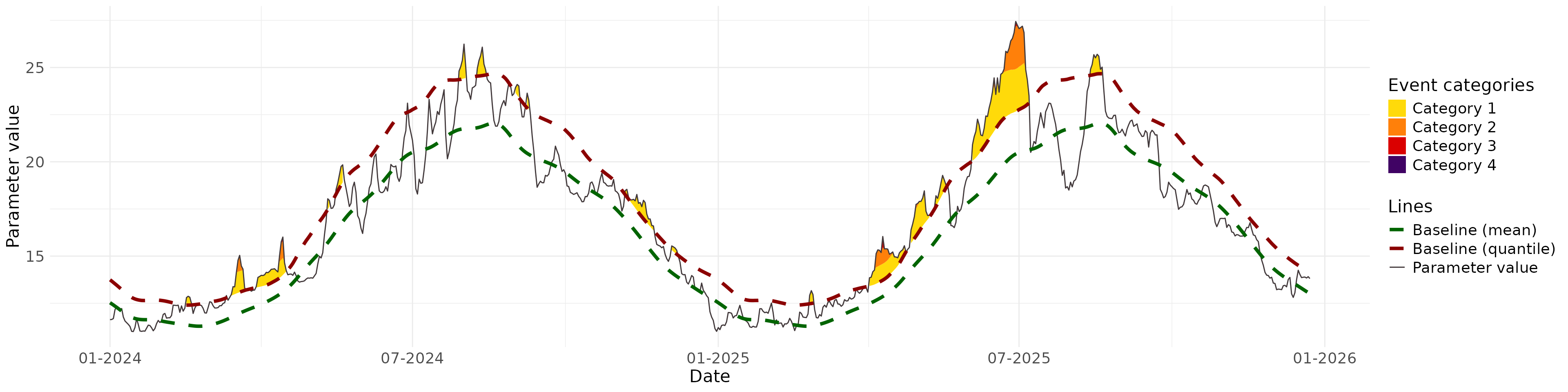
Plot parameters values against the baseline, and the colours indicate the extremes according to the categories:
# get metrics for on gps position
one_place <- metrics_points_day[[2]]

#plot
BEE.plot.categories(metric_point_df = one_place,
                    color_theme = "red",
                    start_date = "2024-01-01",
                    end_date = NULL,
                    # facultative arguments to customise graph:
                    ... = ggplot2::theme(
                              axis.text.x = ggplot2::element_text(size = 14),
                              axis.text.y = ggplot2::element_text(size = 14),
                              axis.title.x = ggplot2::element_text(size = 16),
                              axis.title.y = ggplot2::element_text(size = 16),
                              legend.title =  ggplot2::element_text(size = 16),
                              legend.text  =  ggplot2::element_text(size = 14)
    ))
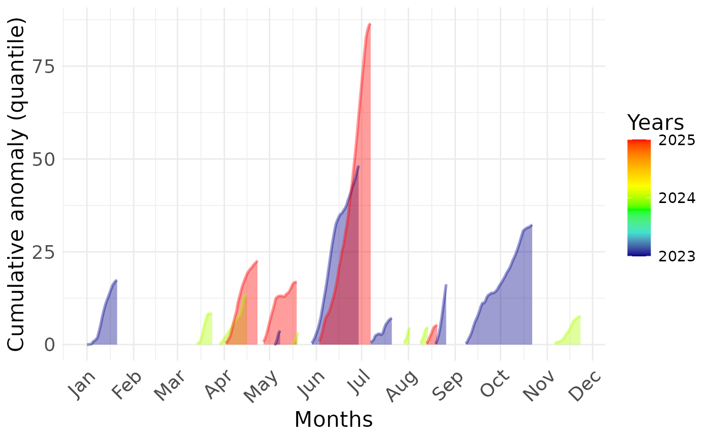
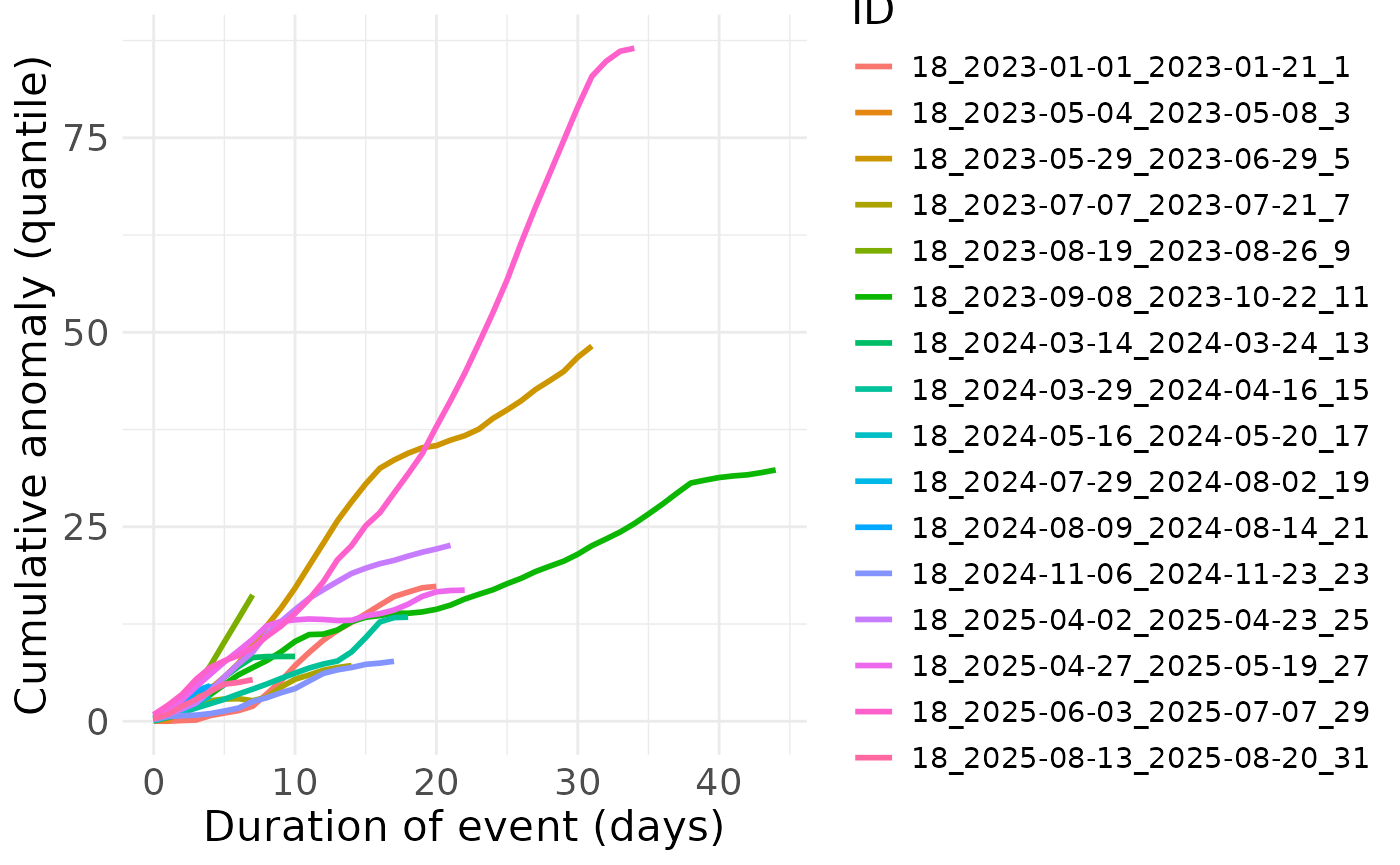
Plot mean value and variance of extreme event:
# get metrics for on gps position
one_place <- metrics_points_day[[2]]

#plot
BEE.plot.cumulative_anomaly(metric_point_df = one_place,
                    start_date = NULL,
                    end_date = NULL,
                    # facultative arguments to customise graph:
                    ... = ggplot2::theme(
                              axis.text.x = ggplot2::element_text(size = 14),
                              axis.text.y = ggplot2::element_text(size = 14),
                              axis.title.x = ggplot2::element_text(size = 16),
                              axis.title.y = ggplot2::element_text(size = 16),
                              legend.title =  ggplot2::element_text(size = 16),
                              legend.text  =  ggplot2::element_text(size = 11)
    ))